

Kafka Streams 101
Another great round by Riccardo Cardin, now a frequent contributor to the Rock the JVM blog. Riccardo is a senior developer, a teacher and a passionate technical blogger. He’s well versed with Apache Kafka; he recently published an article on how to integrate ZIO and Kafka. So now he rolled up his sleeves in the quest of writing the ultimate end-to-end tutorial on Kafka Streams. We hope you enjoy it! Enter Riccardo:
Apache Kafka nowadays is clearly the leading technology concerning message brokers. It’s scalable, resilient, and easy to use. Moreover, it leverages a bunch of exciting client libraries that offer a vast set of additional features. One of these libraries is Kafka Streams.
Kafka Streams brings a complete stateful streaming system based directly on top of Kafka. Moreover, it introduces many exciting concepts, like the duality between topics and database tables. Implementing such ideas, Kafka Streams provides us many valuable operations on topics, such as joins, grouping capabilities, and so on.
Because the Kafka Streams library is quite complex, this article will introduce only its main features, such as the architecture, the Stream DSL with its basic types KStream, KTable, and GlobalKTable, and the transformations defined on them.
1. Set Up
As we said, the Kafka Streams library is implemented using a set of client libraries. In addition, we will use the Circe library to deal with JSON messages. Using Scala as the language to do some experiments, we have to declare the following dependencies in the build.sbt file:
libraryDependencies ++= Seq(
  "org.apache.kafka" % "kafka-clients" % "2.8.0",
  "org.apache.kafka" % "kafka-streams" % "2.8.0",
  "org.apache.kafka" %% "kafka-streams-scala" % "2.8.0",
  "io.circe" %% "circe-core" % "0.14.1",
  "io.circe" %% "circe-generic" % "0.14.1",
  "io.circe" %% "circe-parser" % "0.14.1"
)
Among the dependencies, we find the kafka-streams-scala libraries, a Scala wrapper built around the Java kafka-streams library. In fact, using implicit resolution, the tailored Scala library avoids some boilerplate code.
All the examples we’ll use share the following imports:
import io.circe.generic.auto._
import io.circe.parser._
import io.circe.syntax._
import io.circe.{Decoder, Encoder}
import org.apache.kafka.common.serialization.Serde
import org.apache.kafka.streams.kstream.{GlobalKTable, JoinWindows, TimeWindows, Windowed}
import org.apache.kafka.streams.scala.ImplicitConversions._
import org.apache.kafka.streams.scala._
import org.apache.kafka.streams.scala.kstream.{KGroupedStream, KStream, KTable}
import org.apache.kafka.streams.scala.serialization.Serdes
import org.apache.kafka.streams.scala.serialization.Serdes._
import org.apache.kafka.streams.{KafkaStreams, StreamsConfig, Topology}

import java.time.Duration
import java.time.temporal.ChronoUnit
import java.util.Properties
import scala.concurrent.duration._
We will use version 2.8.0 of Kafka. As we’ve done in the article ZIO Kafka: A Practical Streaming Tutorial, we will start the Kafka broker using a Docker container, declared through a docker-compose.yml file:
version: '2'
services:
  zookeeper:
    image: confluentinc/cp-zookeeper:6.2.0
    hostname: zookeeper
    container_name: zookeeper
    ports:
      - "2181:2181"
    environment:
      ZOOKEEPER_CLIENT_PORT: 2181
      ZOOKEEPER_TICK_TIME: 2000

  kafka:
    image: confluentinc/cp-kafka:6.2.0
    hostname: broker
    container_name: broker
    depends_on:
      - zookeeper
    ports:
      - "29092:29092"
      - "9092:9092"
      - "9101:9101"
    environment:
      KAFKA_BROKER_ID: 1
      KAFKA_ZOOKEEPER_CONNECT: 'zookeeper:2181'
      KAFKA_LISTENER_SECURITY_PROTOCOL_MAP: PLAINTEXT:PLAINTEXT,PLAINTEXT_HOST:PLAINTEXT
      KAFKA_ADVERTISED_LISTENERS: PLAINTEXT://kafka:29092,PLAINTEXT_HOST://localhost:9092
      KAFKA_OFFSETS_TOPIC_REPLICATION_FACTOR: 1
      KAFKA_TRANSACTION_STATE_LOG_MIN_ISR: 1
      KAFKA_TRANSACTION_STATE_LOG_REPLICATION_FACTOR: 1
      KAFKA_GROUP_INITIAL_REBALANCE_DELAY_MS: 0
      KAFKA_JMX_PORT: 9101
      KAFKA_JMX_HOSTNAME: localhost
Please, refer to the above article for further details on starting the Kafka broker inside Docker.
As usual, we need a use case to work with. We’ll try to model some functions concerning the management of orders in an e-commerce site. During the process, we will use the following types:
object Domain {
  type UserId = String
  type Profile = String
  type Product = String
  type OrderId = String

  case class Order(orderId: OrderId, user: UserId, products: List[Product], amount: Double)
  case class Discount(profile: Profile, amount: Double) // in percentage points
  case class Payment(orderId: OrderId, status: String)
}
To set up the application, we also need to create the Kafka topics we will use. In Scala, we represent the topics’ names as constants:
object Topics {
  final val OrdersByUserTopic = "orders-by-user"
  final val DiscountProfilesByUserTopic = "discount-profiles-by-user"
  final val DiscountsTopic = "discounts"
  final val OrdersTopic = "orders"
  final val PaymentsTopic = "payments"
  final val PaidOrdersTopic = "paid-orders"
}
To create such topics in the broker, we use directly the Kafka clients libraries contained in the Docker image:
kafka-topics \
  --bootstrap-server localhost:9092 \
  --topic orders-by-user \
  --create

kafka-topics \
  --bootstrap-server localhost:9092 \
  --topic discount-profiles-by-user \
  --create \
  --config "cleanup.policy=compact"

kafka-topics \
  --bootstrap-server localhost:9092 \
  --topic discounts \
  --create \
  --config "cleanup.policy=compact"

kafka-topics \
  --bootstrap-server localhost:9092 \
  --topic orders \
  --create

kafka-topics \
  --bootstrap-server localhost:9092 \
  --topic payments \
  --create

kafka-topics \
  --bootstrap-server localhost:9092 \
  --topic paid-orders \
  --create
As we can see, we defined some topics as compact. They are a particular type of topic, and we will introduce them deeper during the article.
2. Basics
As we said, the Kafka Streams library is a client library, and it manages streams of messages, reading them from topics and writing the results to different topics.
As we should know, we build streaming applications around three concepts: sources, flows (or pipes), and sinks. Often, we represent streams as a series of tokens, generated by a source, transformed by flows and consumed by sinks:
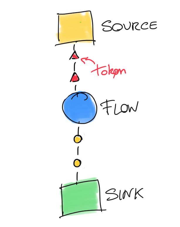
A sources generate the elements that are handled in the stream - here they are the messages read from the topic.
A flow is nothing more than a transformation applied to every token. In functional programming, we represent flows using functions such as map, filter, flatMap, and so on.
Last but not least, a sink is where messages are consumed. After a sink, they don’t exist anymore. In Kafka Streams, sinks can consume messages to a Kafka topic or use anything other technology (i.e., the standard output, a database, etc.)
In Kafka Stream’s jargon, both source, flow, and sink are called stream processors. A streaming application is nothing more than a graph where each node is a processor, and edges are called streams. We can call such a graph a topology.
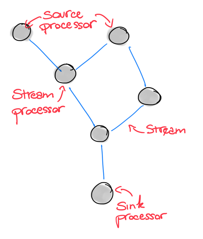
So, with these bullets in our Kafka gun, let’s proceed diving a little deeper into how we can implement some functionalities of our use case scenario using the Kafka Streams library.
3. Messages Serialization and Deserialization
If we want to create any structure on top of Kafka topics, such as stream, we need a standard way to serialize objects into a topic and deserialize messages from topic to objects. The Kafka Streams library uses the so-called Serde type.
What’s a Serde? The Serde word stands for Serializer and Deserializer. A Serde provides the logic to read and write a message from and to a Kafka topic.
So, if we have a Serde[R] instance, we can deserialize and serialize objects of the type R. In this article, we will use JSON format for the payload of Kafka messages. In Scala, one of the most used libraries to marshall and unmarshall JSON into objects is Circe. We already talked about Circe in the post Unleashing the Power of HTTP Apis: The Http4s Library, when we used it together with the Http4s library.
// Scala Kafka Streams library
object Serdes {
  implicit def stringSerde: Serde[String]

  implicit def longSerde: Serde[Long]

  implicit def javaLongSerde: Serde[java.lang.Long]

  // ...
}
In addition, the Serdes object defines the function fromFn, which we can use to build our custom instance of a Serde:
// Scala Kafka Streams library
def fromFn[T >: Null](serializer: T => Array[Byte], deserializer: Array[Byte] => Option[T]): Serde[T]
Wiring all the information together, we can use the above function to create a Serde using Circe:
object Implicits {
  implicit def serde[A >: Null : Decoder : Encoder]: Serde[A] = {
    val serializer = (a: A) => a.asJson.noSpaces.getBytes
    val deserializer = (aAsBytes: Array[Byte]) => {
      val aAsString = new String(aAsBytes)
      val aOrError = decode[A](aAsString)
      aOrError match {
        case Right(a) => Option(a)
        case Left(error) =>
          println(s"There was an error converting the message $aOrError, $error")
          Option.empty
      }
    }
    Serdes.fromFn[A](serializer, deserializer)
  }
}
The serde function constraints the type A to have a Circe Decoder and an Encoder implicitly defined in the scope. Then, it uses the type class Encoder[A] to create a JSON string:
a.asJson
Moreover, the function uses the type class Decoder[A] to parse a JSON string into an object:
decode[A](aAsString)
Fortunately, we can autogenerate Circe Encoder and Decoder type classes importing io.circe.generic.auto._.
Now that we presented the library’s types to write and read from Kafka topics and created some utility functions to deal with such types, we can build our first stream topology.
4. Creating the Topology
First, we need to define the topology of our streaming application. We will use the Stream DSL. This DSL, built on top of the low-level Processor API, is easier to use and master, having a declarative approach. Using the Stream DSL, we don’t have to deal with stream processor nodes directly. The Kafka Streams library will create for us the best processors’ topology reflecting the operation with need.
To create a topology, we need an instance of the builder type provided by the library:
val builder = new StreamsBuilder
The builder lets us create the Stream DSL’s primary types, which are theKStream, Ktable, and GlobalKTable types. Let’s see how.
4.1. Building a KStream
To start, we need to define a source, which will read incoming messages from the Kafka topic orders-by-user we created. Unlike other streaming libraries, such as Akka Streams, the Kafka Streams library doesn’t define any specific type for sources, pipes, and sinks:
val usersOrdersStreams: KStream[UserId, Order] = builder.stream[UserId, Order](OrdersByUserTopic)
We introduced the first notable citizen of the Kafka Streams library: the KStream[K, V] type, representing a regular stream of Kafka messages. Each message has a key of type K and a value of type V.
Moreover, the API to build a new stream looks pretty straightforward because there is a lot of “implicit magic” under the hood. In fact, the full signature of the stream methods is the following:
// Scala Kafka Streams library
def stream[K, V](topic: String)(implicit consumed: Consumed[K, V]): KStream[K, V]
You may wonder what the heck a Consumed[K, V] is. Well, it’s the Java way to provide a Serde for the keys and values of Kafka messages to the stream. Having defined the serde function, we can straightforwardly build a Serde for our Order class. We usually put such classes in the companion object:
object Order {
  implicit val orderSerde: Serde[Order] = serde[Order]
}
However, we can go even further with the implicit generation of the Serde class. In fact, if we define the previous serde function as implicit, the Scala compiler will automatically generate the orderSerde since the Order class fulfills all the needed context bounds.
So, just as a recap, the following implicit resolution took place:
Order => Decoder[Order] / Encoder[Order] => Serde[Order] => Consume[Order]
Why do we need Serde types to be implicit? The main reason is that the Scala Kafka Streams provides the object ImplicitConversions. Inside this object, we find a lot of useful conversion functions that, given Serde objects, let us define a lot of other types, such as the above Consumed. Again, all these conversions save us writing a lot of boilerplate code, which we should have written in Java, for example.
As we said, a KStream[K, V] represents a stream of Kafka messages. This type defines many valuable functions, which we can group into two different families: stateless transformations and stateful transformations. While the former uses only in-memory data structures, the latter requires saving some information inside the so-called state store. We will look at transformations in a minute. But first, we need to introduce the other two basic types of the Stream DSL.
4.2. Building KTable and GlobalKTable
The Kafka Streams library also offers KTable and GlobalKTable, built both on top of a compacted topic. We can think of a compacted topic as a table, indexed by the messages’ key. The broker doesn’t delete messages in a compacted topic using a time to live policy. Every time a new message arrives, a “row” is added to the “table” if the key was not present, or the value associated with the key is updated otherwise. To delete a “row” from the “table”, we just send to the topic a null value associated with the selected key.
As we said in section 1, to make a topic compacted, we need to specify it during its creation:
kafka-topics \
  --bootstrap-server localhost:9092 \
  --topic discount-profiles-by-user \
  --create \
  --config "cleanup.policy=compact"
The above topic will be the starting point to extend our Kafka Streams application. In fact, its messages have a UserId as key and a discount profile as value. A discount profile tells each user which discounts the e-commerce site could apply to the orders of a user. For the sake of simplicity, we represent profiles as simple String:
type Profile = String
Creating a KTable is easy. For example, let’s make a KTable on top of the discount-profiles-by-user topic. Returning to our example, as the users’ number of our e-commerce might be high, we need to partition the information among the nodes of the Kafka cluster. So, let’s create the KTable:
final val DiscountProfilesByUserTopic = "discount-profiles-by-user"

val userProfilesTable: KTable[UserId, Profile] =
  builder.table[UserId, Profile](DiscountProfilesByUserTopic)
As you can imagine, there is more behind the scene than what we can see. Again, using the chain of implicit conversions, the Scala Kafka Streams library creates an instance of the Consumed class, which is mainly used to pass Serde around. In this case, we use the Serdes.stringSerde implicit object, both for the key and the topic’s value.
The methods defined on the KTable type are more or less the same as those on a KStream. In addition, a KTable can be easily converted into a KStream using the following method (or one of its variants):
// Scala Kafka Streams library
def toStream: KStream[K, V]
As we can imagine, creating a GlobalKTable is easy as well. We only need a compacted topic containing a number of keys that is affordable for each cluster node:
kafka-topics \
  --bootstrap-server localhost:9092 \
  --topic discounts \
  --create \
  --config "cleanup.policy=compact"
The number of different instances of discount Profile is low. So. let’s create a GlobalKTable on top of a topic, mapping each discount profile to a discount. First, we define the type modeling a discount:
final val DiscountsTopic = "discounts"

case class Discount(profile: Profile, amount: Double)
Then, we can create an instance of the needed GlobalKTable:
val discountProfilesGTable: GlobalKTable[Profile, Discount] =
  builder.globalTable[Profile, Discount](DiscountsTopic)
Again, under the hood, the library creates an instance of a Consumed object.
So, which is the difference between a KTable and a GlobalKTable? The difference is that a KTable is partitioned between the nodes of the Kafka cluster. However, every node of the cluster receives a full copy of a GlobalKTable. So, be careful with GlobalKTable.
The GlobalKTable type doesn’t define any method. So, why should we ever create an instance of a GlobalKTable? The answer is in the word “joins”. But first, we need to introduce streams transformations.
5. Streams Transformations
Once obtained a KStream or a KTable, we can transform the information they contain using transformations. The Kafka Streams library offers two kinds of transformations: stateless and stateful. While the former executes only in memory, the latter requires managing a state to perform.
5.1. Stateless Transformations
In the group of stateless transformations, we find the classic functions defined on streams, such as filter, map, flatMap, etc. Say, for example, that we want to filter all the orders with an amount greater than 1,000.00 Euro. We can use the filter function (the library also provides a valuable function filterNot):
val expensiveOrders: KStream[UserId, Order] = usersOrdersStreams.filter { (userId, order) =>
  order.amount >= 1000
}
Instead, let’s say that we want to extract a stream of all the purchased products, maintaining the UserId as the message key. Since we want to map only the values of the Kafka messages, we can use the mapValues function:
val purchasedListOfProductsStream: KStream[UserId, List[Product]] = usersOrdersStreams.mapValues { order =>
  order.products
}
Going further, we can obtain a KStream[UserId, Product] instead, just using the flatMapValues function:
val purchasedProductsStream: KStream[UserId, Product] = usersOrdersStreams.flatMapValues { order =>
  order.products
}
Moreover, the library contains stateless terminal transformations, called sinks, representing a terminal node of our stream topology. We can apply no other function to the stream after a sink is reached. Two examples of sink processors are the foreach and to methods.
The foreach method applies to a stream a given function:
// Scala Kafka Streams library
def foreach(action: (K, V) => Unit): Unit
As an example, imagine we want to print all the products purchased by a user. We can call the ` foreach method directly on the purchasedProductsStream` stream:
purchasedProductsStream.foreach { (userId, product) =>
  println(s"The user $userId purchased the product $product")
}
Another interesting sink processor is the to method, which persists the messages of the stream into a new topic:
expensiveOrders.to("suspicious-orders")
In the above example, we are writing all the orders greater than 1,000.00 Euro in a dedicated topic, probably performing fraud analysis. Again, the Scala Kafka Streams library saves us from typing a lot of code. In fact, the full signature of the to method is the following:
// Scala Kafka Streams library
def to(topic: String)(implicit produced: Produced[K, V]): Unit
The implicit instance of the Produced type, which is a wrapper around key and value Serde, is produced automatically by the functions in the ImplicitConversions object, plus our serde implicit function.
Last but not least, we have grouping, which groups different values under the same key. We group values maintaining the original key using the groupByKey transformation:
// Scala Kafka Streams library
def groupByKey(implicit grouped: Grouped[K, V]): KGroupedStream[K, V]
As usual, the Grouped object carries the Serde types for keys and values, and it’s automatically derived by the compiler if we use the Scala Kafka Streams library.
For example, imagine we want to group the purchasedProductsStream to perform some aggregated operation later. In detail, we want to group each user with the purchased products:
val productsPurchasedByUsers: KGroupedStream[UserId, Product] = purchasedProductsStream.groupByKey
As we may notice, we introduced a new type of stream, the KGroupedStream. This type defines only stateful transformation on it. So, for this reason, we say that grouping is the precondition to stateful transformations.
Moreover, if we want to group a stream using something that is not the messages’ keys, we can use the groupBy transformation:
val purchasedByFirstLetter: KGroupedStream[String, Product] =
  purchasedProductsStream.groupBy[String] { (userId, products) =>
    userId.charAt(0).toLower.toString
  }
In the above example, we group products by the first letter of the UserId of the user who purchased them. It seems a harmless operation from the code, as we are only changing the stream’s key. However, since Kafka partitioned topics by key, the change of the key marks the topic for re-partitioning.
So, suppose the marked stream will be materialized in a topic or in a state store (more to come on state stores) by the following transformation. In that case, the contained messages will be potentially moved to another node of the Kafka cluster. Re-partitioning is an operation that should be done with caution because it could generate a heavy network load.
5.2. Stateful Transformations
As the name of these types of transformations suggested, the Kafka Streams library needs to maintain some kind of state to manage them, and it’s called state store. The state store, which is automatically controlled by the library if we use the Stream DSL, can be an in-memory hashmap or an instance of RocksDB, or any other convenient data structure.
Each state store is local to the node containing the instance of the stream application and refers to the messages concerning the partitions owned by the node. So, the global state of a stream application is the sum of all the states of the single node. Kafka Streams offers fault-tolerance and automatic recovery for local state stores.
Now that we know about the existence of state stores, we can start talking about stateful transformations. There are many of them, such as:
- Aggregations
- Aggregations using windowing
- Joins
Joins are considered stateful transformations too, but we will treat joins in a dedicated section. However, we can make some examples of aggregations. Aggregations are key-based operations, which means that they always operate over records of the same key.
As we saw, we previously obtained a KGroupedStream containing the products purchased by users:
val productsPurchasedByUsers: KGroupedStream[UserId, Product] = purchasedProductsStream.groupByKey
Now, we can count how many products each user purchased by calling the count transformation:
val numberOfProductsByUser: KTable[UserId, Long] = productsPurchasedByUsers.count()
Since the number of purchased products by users updates every time a new message is available, the result of the count transformation is a KTable, which will update during time accordingly.
The count transformation uses the implicit parameters’ resolution we just saw. In fact, its signature is the following:
// Scala Kafka Stream library
def count()(implicit materialized: Materialized[K, Long, ByteArrayKeyValueStore]): KTable[K, Long]
As for the Consumed implicit objects, the implicit Materialized[K, V, S] instance is directly derived by the compiler from the available implicit instances of key and value Serde.
The count transformation is not the only aggregation type in the Kafka Streams library, offering generic aggregations. Since simple aggregations are very similar to the example we associated with the count transformation, we now introduce windowed aggregations instead.
In detail, the Kafka Streams library lets us aggregate messages using a time window. All the messages that arrived inside the window are eligible for being aggregated. Clearly, we are talking about a sliding window through time. The library allows us to aggregate using different types of windows, each one with its own features. Since windowing is a complex issue, we will not go deeper into it in this article.
For our example, we will use Tumbling time windows. They model fixed-size, non-overlapping, gap-less windows. In detail, we want to know how many products our users purchase every ten seconds. First, we need to create the window representation:
val everyTenSeconds: TimeWindows = TimeWindows.of(10.second.toJava)
Then, we use it to define our windowed aggregation:
val numberOfProductsByUserEveryTenSeconds: KTable[Windowed[UserId], Long] =
  productsPurchasedByUsers.windowedBy(everyTenSeconds)
    .aggregate[Long](0L) { (userId, product, counter) =>
      counter + 1
    }
As for the count transformation, the final result is a Ktable. However, this time we have a Windowed[UserId] as the key type, a convenient type containing both the key and the lower and upper bound of the window.
The Scala Kafka Streams library defines the aggregate transformation as the Scala language defines the foldLeft method on sequences. The first parameter is the starting accumulation point, and the second is the folding function. Finally, an implicit instance of a Materialized[K, V, S] object is automatically derived by the compiler:
// Scala Kafka Stream library
def aggregate[VR](initializer: => VR)(aggregator: (K, V, VR) => VR)(
  implicit materialized: Materialized[K, VR, ByteArrayWindowStore]
): KTable[Windowed[K], VR]
The library defines many other stateful transformations. Please, refer to the official documentation that lists all of them.
6. Joining Streams
In my opinion, the most essential feature of the Kafka Streams library is the ability to join streams. The Kafka team strongly supports the duality between streams and database tables. To keep it simple, we can view a stream as the changelog of a database table, whose primary keys are equal to the keys of the Kafka messages.
Following this duality, we can think about records in a KStream as they are INSERT operations on a table. In fact, for the nature of a KStream, every message is different from any previous message. Instead, a KTable is an abstraction of a changelog stream, where each record represents an UPSERT: If the key is not present in the table, the record is equal to an INSERT, and an UPDATE otherwise.
With these concepts in mind, it’s easier for us to accept the existence of joins between Kafka Streams.
As we already said, joins are stateful operations, requiring a state store to execute.
6.1. Joining a KStream and a KTable
The most accessible kind of join is between a KStream and a KTable. The join operation is on the keys of the messages. The broker has to ensure that the data is co-partitioned. To go deeper into co-partitioning, please refer to Joining. To put it simply, if data of two topics are co-partitioned, then the Kafka broker can ensure the joining message resides on the same node of the cluster, avoiding shuffling of messages between nodes.
Returning to our leading example, imagine we want to join the orders stream, which is indexed by UserId, with the table containing the discount profile of each user:
val ordersWithUserProfileStream: KStream[UserId, (Order, Profile)] =
  usersOrdersStreams.join[Profile, (Order, Profile)](userProfilesTable) { (order, profile) =>
    (order, profile)
  }
As we have seen in many cases, the Scala Kafka Streams library saves us from typing a lot of boilerplate code, implicitly deriving the type that carries the Serde information:
// Scala Kafka Stream library
def join[VT, VR](table: KTable[K, VT])(joiner: (V, VT) => VR)(implicit joined: Joined[K, V, VT]): KStream[K, VR]
The first method’s parameter is the KTable, whereas the second is a function that returns a new value of any type given the pair of the joined values.
In our use case, the join produces a stream containing all the orders purchased by each user, added with the discount profile information. So, the result of a join is a set of messages having the same key as the originals and a transformation of the joined messages’ payloads as value.
6.2. Joining with a GlobalKTable
Another type of join is between a KStream (or a KTable) and a GlobalKTable. As we said, the broker replicates the information of a GlobalKTable in each cluster node. So, we don’t need the co-partitioning property anymore because the broker ensures the locality of GlobalKTable messages for all the nodes.
In fact, the signature of this type of join transformation is different from the previous:
// Scala Kafka Stream library
def join[GK, GV, RV](globalKTable: GlobalKTable[GK, GV])(
  keyValueMapper: (K, V) => GK,
  joiner: (V, GV) => RV,
): KStream[K, RV]
The keyValueMapper input function maps the information of the stream in the key GK of GlobalKTable. In this case, we can use any helpful information in the message, both the key and the payload. Instead, the transformation uses the joiner function to extract the new payload.
In our example, we can use a join between the stream ordersWithUserProfileStream and the global table discountProfilesGTable to obtain a new stream with the amount of the discounted order, using the discount associated with the profile of a UserId:
val discountedOrdersStream: KStream[UserId, Order] =
  ordersWithUserProfileStream.join[Profile, Discount, Order](discountProfilesGTable)(
    { case (_, (_, profile)) => profile }, // Joining key
    { case ((order, _), discount) => order.copy(amount = order.amount * discount.amount) }
  )
Obtaining the joining key is easy: We just select the Profile information contained in the messages’ payload of the stream ordersWithUserProfileStream. Then, the new value of each message is the discounted amount.
6.3. Joining KStreams
Last but not least, we have another type of join transformation, maybe the most interesting. We’re talking about the join between two streams.
In the joins we’ve seen so far, one of the two joining operands always represented a table, which means a persistent form of information. Once a key enters the table, it will be present in it until someone removes it. So, Joining with a table reduces to make a lookup in table’s keys for every message in the stream.
However, streams are continuously changing pieces of information. So, how can we join such volatile data? Once again, windowing comes into help. The join transformation between two streams joins messages by key. Moreover, messages must arrive at the topics within a sliding window of time. Besides, the data must be co-partitioned for the join between KStream and KTable.
Since joins are stateful transformations, we must window the join between two streams; otherwise, the underlining state store would grow indefinitely.
Moreover, the semantics of stream-stream join is that a new input record on one side will produce a join output for each matching record on the other side, and there can be multiple such matching records in a given join window.
Talking about purchased orders, imagine we want to join the stream of discounted orders with stream listing orders that received payment, obtaining a stream of paid orders. First, we need to define the latter stream built upon the topic called payments. Moreover, we define the Payment type that associates each OrderId with its payment status:
val paymentsStream: KStream[OrderId, Payment] = builder.stream[OrderId, Payment](PaymentsTopic)
It’s reasonable that the payment of the order arrives at most some minutes after the order itself. So, it seems that we have a perfect use case to apply the join between streams. But first, we need to change the key of the discountedOrdersStream to an OrderId. Fortunately, the library offers the transformation called selectKey:
val ordersStream: KStream[OrderId, Order] = discountedOrdersStream.selectKey { (_, order) => order.orderId }
We have to pay attention when we change the key of a stream. In fact, the broker needs to move the messages among nodes to ensure the co-partitioning constraint. This operation is called shuffling, and it’s very time and resource-consuming.
The ordersStream stream represents the same information as the discountedOrdersStream, but is indexed by OrderId. Now, we’ve met the preconditions to join our streams:
val paidOrders: KStream[OrderId, Order] = {

  val joinOrdersAndPayments = (order: Order, payment: Payment) =>
    if (payment.status == "PAID") Option(order) else Option.empty[Order]

  val joinWindow = JoinWindows.of(Duration.of(5, ChronoUnit.MINUTES))

  ordersStream.join[Payment, Option[Order]](paymentsStream)(joinOrdersAndPayments, joinWindow)
    .flatMapValues(maybeOrder => maybeOrder.toIterable)
}
The final stream, paidOrders, contains all the orders paid at most five minutes after their arrival into the application. As we can see, we applied a joining sliding window of five minutes:
val joinWindow = JoinWindows.of(Duration.of(5, ChronoUnit.MINUTES))
As the stream-stream join uses the key of the messages, we only need to provide the mapping function of the joined values, other than the joining window.
To explain the semantic of the join, we can look at the following table. The first column mimics the passing of time, while the following two columns represent the values of the messages in the two starting streams. For the sake o simplicity, the key, aka the OrderId, is the same for all the messages. Moreover, the table represents a five minutes window, starting from the arrival of the first message:
| Timestamp | ordersStream |
paymentsStream |
Joined value |
|---|---|---|---|
| 1 | Order("order1") |
||
| 2 | Payment("REQUESTED") |
Option.empty |
|
| 3 | Payment("ISSUED") |
Option.empty |
|
| 4 | Payment("PAID") |
Some(Order) |
At time 1, we receive the discounted order with id order1. From time 2 to 4, we get three messages into the paymentsStream for the same order, representing three different payment statuses. All three messages will join the order since we received them inside the defined window.
The three types of join transformation we presented represent only the primary examples of the joins available in the Kafka Streams library. In fact, the library offers to developers also left join and outer joins, but their description is far beyond the scope of this article.
7. The Kafka Streams Application
Once we have defined the desired topology for our application, it’s time to materialize and execute it. Materializing the topology is easy since we only have to call the build method on the instance of the StreamBuilder we have used so far:
val topology: Topology = builder.build()
The object of type Topology represents the whole set of transformations we defined. Interestingly, we can also print the topology simply calling the describe method on it and obtaining a TopologyDescription description object that is suitable for printing:
println(topology.describe())
The printed topology of our leading example is the following:
Topologies:
   Sub-topology: 0
    Source: KSTREAM-SOURCE-0000000000 (topics: [orders-by-user])
      --> KSTREAM-JOIN-0000000007
    Processor: KSTREAM-JOIN-0000000007 (stores: [discount-profiles-by-user-STATE-STORE-0000000001])
      --> KSTREAM-LEFTJOIN-0000000008
      <-- KSTREAM-SOURCE-0000000000
    Processor: KSTREAM-LEFTJOIN-0000000008 (stores: [])
      --> KSTREAM-KEY-SELECT-0000000009
      <-- KSTREAM-JOIN-0000000007
    Processor: KSTREAM-KEY-SELECT-0000000009 (stores: [])
      --> KSTREAM-FILTER-0000000012
      <-- KSTREAM-LEFTJOIN-0000000008
    Processor: KSTREAM-FILTER-0000000012 (stores: [])
      --> KSTREAM-SINK-0000000011
      <-- KSTREAM-KEY-SELECT-0000000009
    Source: KSTREAM-SOURCE-0000000002 (topics: [discount-profiles-by-user])
      --> KTABLE-SOURCE-0000000003
    Sink: KSTREAM-SINK-0000000011 (topic: KSTREAM-KEY-SELECT-0000000009-repartition)
      <-- KSTREAM-FILTER-0000000012
    Processor: KTABLE-SOURCE-0000000003 (stores: [discount-profiles-by-user-STATE-STORE-0000000001])
      --> none
      <-- KSTREAM-SOURCE-0000000002

  Sub-topology: 1 for global store (will not generate tasks)
    Source: KSTREAM-SOURCE-0000000005 (topics: [discounts])
      --> KTABLE-SOURCE-0000000006
    Processor: KTABLE-SOURCE-0000000006 (stores: [discounts-STATE-STORE-0000000004])
      --> none
      <-- KSTREAM-SOURCE-0000000005
  Sub-topology: 2
    Source: KSTREAM-SOURCE-0000000010 (topics: [payments])
      --> KSTREAM-WINDOWED-0000000015
    Source: KSTREAM-SOURCE-0000000013 (topics: [KSTREAM-KEY-SELECT-0000000009-repartition])
      --> KSTREAM-WINDOWED-0000000014
    Processor: KSTREAM-WINDOWED-0000000014 (stores: [KSTREAM-JOINTHIS-0000000016-store])
      --> KSTREAM-JOINTHIS-0000000016
      <-- KSTREAM-SOURCE-0000000013
    Processor: KSTREAM-WINDOWED-0000000015 (stores: [KSTREAM-JOINOTHER-0000000017-store])
      --> KSTREAM-JOINOTHER-0000000017
      <-- KSTREAM-SOURCE-0000000010
    Processor: KSTREAM-JOINOTHER-0000000017 (stores: [KSTREAM-JOINTHIS-0000000016-store])
      --> KSTREAM-MERGE-0000000018
      <-- KSTREAM-WINDOWED-0000000015
    Processor: KSTREAM-JOINTHIS-0000000016 (stores: [KSTREAM-JOINOTHER-0000000017-store])
      --> KSTREAM-MERGE-0000000018
      <-- KSTREAM-WINDOWED-0000000014
    Processor: KSTREAM-MERGE-0000000018 (stores: [])
      --> KSTREAM-FLATMAPVALUES-0000000019
      <-- KSTREAM-JOINTHIS-0000000016, KSTREAM-JOINOTHER-0000000017
    Processor: KSTREAM-FLATMAPVALUES-0000000019 (stores: [])
      --> KSTREAM-SINK-0000000020
      <-- KSTREAM-MERGE-0000000018
    Sink: KSTREAM-SINK-0000000020 (topic: paid-orders)
      <-- KSTREAM-FLATMAPVALUES-0000000019
The above text representation is a bit hard to read – fortunately, there’s an open-source project which can create a visual graph of the topology, starting from the above output. The project is called kafka-stream-viz, and the generated visual graph for our topology is the following:
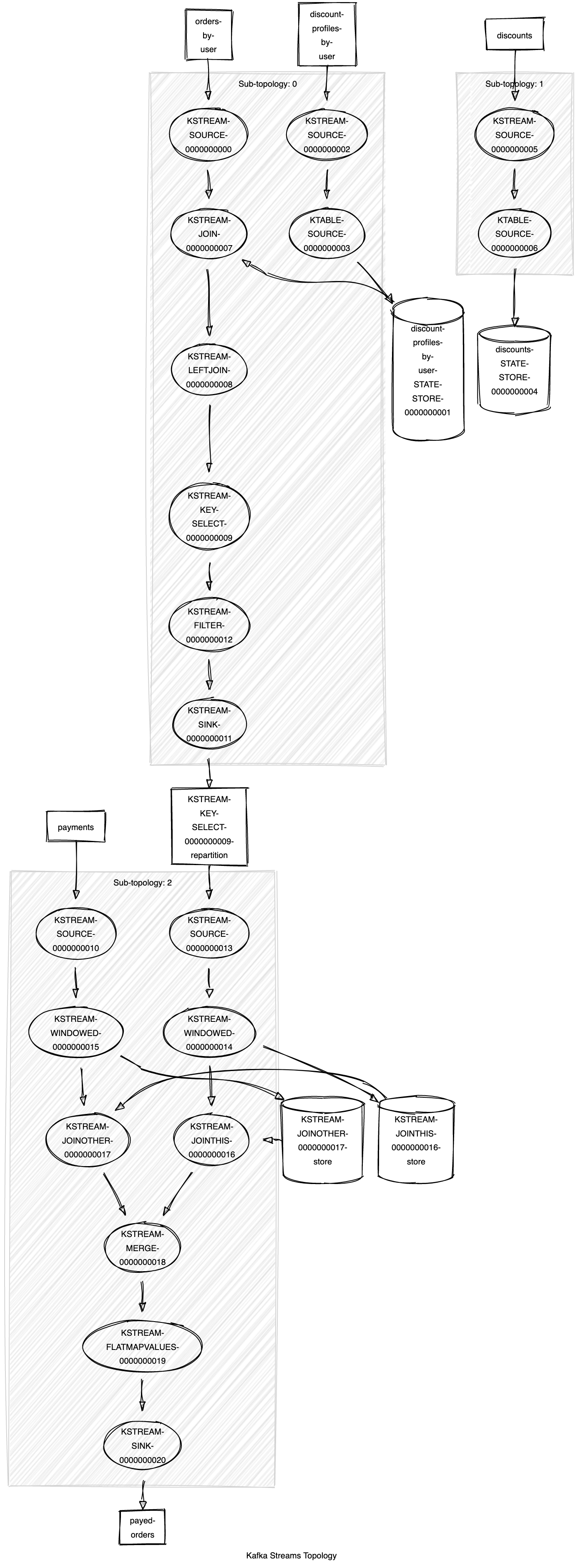
This graphical representation allows us to follow the sequences of transformations easier than the text form. In addition, it becomes straightforward to understand which transformation is stateful and so requires a state store.
Once we materialize the topology, we can effectively run the Kafka Streams application. First, we have to set the url to connect to the Kafka cluster, and the name of the application:
val props = new Properties
props.put(StreamsConfig.APPLICATION_ID_CONFIG, "orders-application")
props.put(StreamsConfig.BOOTSTRAP_SERVERS_CONFIG, "localhost:9092")
props.put(StreamsConfig.DEFAULT_KEY_SERDE_CLASS_CONFIG, Serdes.stringSerde.getClass)
In our example, we also configured the default Serde type for keys. Then, the last step is to create the KafkaStream application and start it:
val application: KafkaStreams = new KafkaStreams(topology, props)
application.start()
Finally, the complete application for the leading example of our article, which leads to paid orders, is the following:
object KafkaStreamsApp {

  implicit def serde[A >: Null : Decoder : Encoder]: Serde[A] = {
    val serializer = (a: A) => a.asJson.noSpaces.getBytes
    val deserializer = (aAsBytes: Array[Byte]) => {
      val aAsString = new String(aAsBytes)
      val aOrError = decode[A](aAsString)
      aOrError match {
        case Right(a) => Option(a)
        case Left(error) =>
          println(s"There was an error converting the message $aOrError, $error")
          Option.empty
      }
    }
    Serdes.fromFn[A](serializer, deserializer)
  }

  // Topics
  final val OrdersByUserTopic = "orders-by-user"
  final val DiscountProfilesByUserTopic = "discount-profiles-by-user"
  final val DiscountsTopic = "discounts"
  final val OrdersTopic = "orders"
  final val PaymentsTopic = "payments"
  final val PayedOrdersTopic = "paid-orders"

  type UserId = String
  type Profile = String
  type Product = String
  type OrderId = String

  case class Order(orderId: OrderId, user: UserId, products: List[Product], amount: Double)

  // Discounts profiles are a (String, String) topic

  case class Discount(profile: Profile, amount: Double)

  case class Payment(orderId: OrderId, status: String)

  val builder = new StreamsBuilder

  val usersOrdersStreams: KStream[UserId, Order] = builder.stream[UserId, Order](OrdersByUserTopic)

  def paidOrdersTopology(): Unit = {
    val userProfilesTable: KTable[UserId, Profile] =
      builder.table[UserId, Profile](DiscountProfilesByUserTopic)

    val discountProfilesGTable: GlobalKTable[Profile, Discount] =
      builder.globalTable[Profile, Discount](DiscountsTopic)

    val ordersWithUserProfileStream: KStream[UserId, (Order, Profile)] =
      usersOrdersStreams.join[Profile, (Order, Profile)](userProfilesTable) { (order, profile) =>
        (order, profile)
      }

    val discountedOrdersStream: KStream[UserId, Order] =
      ordersWithUserProfileStream.join[Profile, Discount, Order](discountProfilesGTable)(
        { case (_, (_, profile)) => profile }, // Joining key
        { case ((order, _), discount) => order.copy(amount = order.amount * discount.amount) }
      )

    val ordersStream: KStream[OrderId, Order] = discountedOrdersStream.selectKey { (_, order) => order.orderId }

    val paymentsStream: KStream[OrderId, Payment] = builder.stream[OrderId, Payment](PaymentsTopic)

    val paidOrders: KStream[OrderId, Order] = {

      val joinOrdersAndPayments = (order: Order, payment: Payment) =>
        if (payment.status == "PAID") Option(order) else Option.empty[Order]

      val joinWindow = JoinWindows.of(Duration.of(5, ChronoUnit.MINUTES))

      ordersStream.join[Payment, Option[Order]](paymentsStream)(joinOrdersAndPayments, joinWindow)
        .flatMapValues(maybeOrder => maybeOrder.toIterable)
    }

    paidOrders.to(PayedOrdersTopic)
  }

  def main(args: Array[String]): Unit = {
    val props = new Properties
    props.put(StreamsConfig.APPLICATION_ID_CONFIG, "orders-application")
    props.put(StreamsConfig.BOOTSTRAP_SERVERS_CONFIG, "localhost:9092")
    props.put(StreamsConfig.DEFAULT_KEY_SERDE_CLASS_CONFIG, Serdes.stringSerde.getClass)

    paidOrdersTopology()

    val topology: Topology = builder.build()

    println(topology.describe())

    val application: KafkaStreams = new KafkaStreams(topology, props)
    application.start()
  }
}
And, that’s all about the Kafka Streams library, folks!
8. Let’s Run It
At this point, we defined a complete working Kafka application, which uses many transformations and joins. Now, it’s time to test the developed topology, sending messages to the various Kafka topics.
First, let’s fill the tables, starting from the topic discounts. We have to send some messages associating a profile with a discount:
kafka-console-producer \
   --topic discounts \
   --broker-list localhost:9092 \
   --property parse.key=true \
   --property key.separator=,
<Hit Enter>
profile1,{"profile":"profile1","amount":0.5 }
profile2,{"profile":"profile2","amount":0.25 }
profile3,{"profile":"profile3","amount":0.15 }
We created three profiles in the above command with a discount of 50%, 25%, and 15%, respectively.
The next step is to create some users and associated them with a discount profile in the topic discount-profiles-by-user:
kafka-console-producer \
   --topic discount-profiles-by-user \
   --broker-list localhost:9092 \
   --property parse.key=true \
   --property key.separator=,
<Hit Enter>
Daniel,profile1
Riccardo,profile2
We are ready to insert our first order into the system, using the topic orders-by-user. As the name of the topic said, the keys of the following messages are user-ids:
kafka-console-producer \
   --topic orders-by-user \
   --broker-list localhost:9092 \
   --property parse.key=true \
   --property key.separator=,
<Hit Enter>
Daniel,{"orderId":"order1","user":"Daniel","products":[ "iPhone 13","MacBook Pro 15"],"amount":4000.0 }
Riccardo,{"orderId":"order2","user":"Riccardo","products":["iPhone 11"],"amount":800.0}
Now, we must pay the above orders. So, we send the messages representing the payment transaction. The topic storing such messages is called payments:
kafka-console-producer \
   --topic payments \
   --broker-list localhost:9092 \
   --property parse.key=true \
   --property key.separator=,
<Hit Enter>
order1,{"orderId":"order1","status":"PAID"}
order2,{"orderId":"order2","status":"PENDING"}
If everything goes right, into the topic paid-orders we should find a message containing the paid order of the user "Daniel", containing an "iPhone 13" and a "MacBook Pro 15", and worth 2,000.0 Euro. We can read the messages of the topic using the kafka-console-consumer.sh shell command:
kafka-console-consumer \
    --bootstrap-server localhost:9092 \
    --topic paid-orders \
    --from-beginning
The above command will read the following message, concluding our journey in the Kafka Streams library:
{"orderId":"order1","user":"Daniel","products":["iPhone 13","MacBook Pro 15"],"amount":2000.0}
9. Conclusions
This article introduced the Kafka Streams library, a Kafka client library based on top of the Kafka consumers and producers API. In detail, we focused on the Stream DSL part of the library, which lets us represent the stream’s topology at a higher level of abstraction. After introducing the basic building blocks of the DSL, KStream, KTable, and GlobalKTable, we showed the primary operations defined on them, both the stateless and the stateful ones. Then, we talked about joins, one of the most relevant features of Kafka Streams. Finally, we wired all together, and we learned how to start a Kafka Streams application.
The Kafka Streams library is vast, and it offers many more features than we saw. For example, we’ve not talked about the Processor API and how it’s possible to query a state store directly. However, the given information should be sufficient to have a solid base to learn the advanced feature of the excellent and helpful library.